SIMPLE tutorial
%load_ext autoreload
%autoreload 2
import matplotlib.pyplot as plt
%matplotlib inline

# update matplotlib params for bigger font
import matplotlib.pylab as pylab
params = {'mathtext.fontset': 'stix',
         'font.family': 'STIXGeneral'}
pylab.rcParams.update(params)
from simple.simple import LognormalIntensityMock
from astropy.cosmology import Planck18 as cosmo
import astropy.units as u
import astropy.constants as const
from astropy.table import Table

import numpy as np
import yaml
import os

from scipy.integrate import quad
Run manually
Define the luminosity function
The function has to be dimensionless, i.e. the input is given in units
of the defined luminosity_unit and the output will be in units of
\(\frac{1}{\mathrm{Mpc}^3\mathrm{luminosity\_unit}}\). It is best to
use a typical luminosity for luminosity_unit so that the numerical
errors of the integration will be small.
luminosity_unit = 1e42 * u.erg / u.s

def luminosity_function(L):
    """
    Calculates dn/dL (L), where L must be in units of luminosity_unit.
    For integration purposes, make sure that L/luminosity_unit is typically
    a small number, so that the numbers don't overflow in the integration.
    For example, luminosity_unit could be the mean expected luminosity.

    Luminosity function from Konno et al. (2016).
    """
    Lstar = (4.87 * luminosity_unit).to(luminosity_unit).value # 1e42 erg / s
    phistar = 3.37 * 1e-4 # Mpc-3
    alpha = -1.8

    return phistar * (L/Lstar)**alpha * np.exp(-L/Lstar) * 1/Lstar
We will save the luminosity function in a table so that we can later
initiate the LognormalIntensityMock instance from files.
max_L_for_saving = 1e45 * u.erg / u.s
Lmin = 1e40 * u.erg / u.s
if np.isfinite(max_L_for_saving):
    max_log10_L_for_saving = np.log10(
        max_L_for_saving.to(luminosity_unit).value)
else:
    max_log10_L_for_saving = np.log10((1e5 * Lmin).to(luminosity_unit).value)
min_log10_L_for_saving = np.log10(Lmin.to(luminosity_unit).value)
N_save = 10000
dlog_10_L = (max_log10_L_for_saving - min_log10_L_for_saving) / N_save
log_10_Ls = np.linspace(min_log10_L_for_saving, max_log10_L_for_saving, N_save)

lum_tab = Table()
lum_tab["L"] = 10**log_10_Ls
lum_tab["dn/dL"] = luminosity_function(10**log_10_Ls)
lum_tab.write("luminosity_function_example.csv",
              format="csv", overwrite=True)
Set up input parameters
It is possible to initiate a LognormalIntensityMock instance from a
dictionary or from a yaml file that contains this dictionary.
input_dict = {"verbose" : False,
              "bias" : 1.5,
              "redshift" : 2.0,
              "single_redshift" : False,
              "box_size" : np.array([400,400,400]) * u.Mpc,
              "N_mesh" : np.array([128,128,128]),
              "luminosity_unit" : luminosity_unit,
              "Lmin" : 2e41 * u.erg/u.s,
              "Lmax" : np.inf * u.erg/u.s,
              "galaxy_selection" : {"intensity" : "all",
                                    "n_gal" : "detected"},
              "lambda_restframe" : 1215.67 * u.angstrom,
              "brightness_temperature" : False,
              "do_spectral_smooth" : True,
              "do_spectral_tophat_smooth" : False,
              "do_angular_smooth" : True,
              "sigma_beam" : 6 * u.arcsec,
              "dlambda" : 5 * u.angstrom,
              "footprint_radius" : 9 * u.arcmin,
              "luminosity_function" : luminosity_function,
              "run_pk" : {"intensity": True,
                        "n_gal": True,
                        "cross": True,
                        "sky_subtracted_cross": True
                            },
              "dk" : 0.04,
              "kmin" : 0.04,
              "kmax" : 1.0,
              "seed_lognormal" : 100,
              "outfile_prefix" : 'mock',
              "cosmology" : cosmo,
              "lnAs" : 3.094,
              "n_s" : 0.9645,
              "RSD" : True,
              "out_dir" : "../tmp/mocks/",
              "min_flux" : 3e-17 * u.erg/u.s/u.cm**2,
              "sigma_noise" : 2e-22 * u.erg/u.s/u.cm**2/u.angstrom/u.arcsec**2,
}
Initiate the LognormalIntensityMock instance
with the input dictionary:
lim = LognormalIntensityMock(input_dict)
Or initiate the LognormalIntensityMock instance from a yaml file
that contains the input dictionary. In this case, the cosmology must be
specified in a file or a dictionary that can be evaluated by astropy to
construct a cosmology object or as a string that is part of the astropy
cosmology collection, such as Planck18. The luminosity function also
has to be specified as the name of the file that contains the tabulated
luminosity function.
lim = LognormalIntensityMock("example_input_file.yaml")
2023-07-14 14:15:06,282 simple WARNING: We extrapolate the values outside of the provided tabulated values of L.
Plot plt.loglog(Ls, lim.luminosity_function(Ls)) in a reasonable range to check the outcome!
Run the lognormal galaxy simulation from lognognormal_galaxies and load the catalog:
lim.run_lognormal_simulation_cpp()
lim.load_lognormal_catalog_cpp(
                bin_filename=lim.lognormal_bin_filename)
[0.   0.   0.06] eV
{'ofile_prefix': 'mock', 'inp_pk_fname': '../tmp/mocks/inputs/mock_pk.txt', 'xi_fname': '../tmp/mocks/inputs/mock_Rh_xi.txt', 'pkg_fname': '../tmp/mocks/inputs/mock_pkG.dat', 'mpkg_fname': '../tmp/mocks/inputs/mock_mpkG.dat', 'cpkg_fname': '../tmp/mocks/inputs/mock_mpkG.dat', 'f_fname': '../tmp/mocks/inputs/mock_fnu.txt', 'z': 2.0, 'mnu': 0.06, 'oc0h2': 0.11934063901639999, 'ob0h2': 0.0224178568132, 'ns': 0.9645, 'lnAs': 3.094, 'h0': <Quantity 0.6766>, 'w': -1.0, 'run': 0.0, 'bias': 1.5, 'bias_mpkG': 1.0, 'bias_cpkG': 1.35, 'Nrealization': 1, 'Ngalaxies': 279657, 'Lx': 270.64000000000004, 'Ly': 270.64000000000004, 'Lz': 270.64000000000004, 'rmax': 10000.0, 'seed': 100, 'Pnmax': 128, 'losy': 0.0, 'losz': 0.0, 'kbin': 0.01, 'kmax': 0.0, 'lmax': 4, 'gen_inputs': True, 'run_lognormal': True, 'calc_pk': False, 'calc_cpk': False, 'use_cpkG': 0, 'output_matter': 0, 'output_gal': 1, 'calc_mode_pk': 0, 'out_dir': '../tmp/mocks/', 'halofname_prefix': '', 'imul_fname': '', 'num_para': 1, 'om0h2': 0.14175849582959998, 'om0': 0.30966, 'ob0': 0.04897, 'ode0': 0.6888463055445441, 'losx': 1.0, 'As': 2.2065162338947054e-09, 'aH': 100.27554429639554}
dir_name:  ../tmp/mocks/
../tmp/mocks/rsd
../tmp/mocks/realspace
dir_name:  ../tmp/mocks/inputs
../tmp/mocks/inputs/rsd
../tmp/mocks/inputs/realspace
dir_name:  ../tmp/mocks/lognormal
../tmp/mocks/lognormal/rsd
../tmp/mocks/lognormal/realspace
dir_name:  ../tmp/mocks/pk
../tmp/mocks/pk/rsd
../tmp/mocks/pk/realspace
dir_name:  ../tmp/mocks/coupling
../tmp/mocks/coupling/rsd
../tmp/mocks/coupling/realspace
time ~/Documents/projects/playground/lognormal_galaxies/eisensteinhubaonu/compute_pk ../tmp/mocks//inputs/mock 0.30966 0.6888463055445441 0.04897 0.6766 -1.0 0.9645 0.0 2.2065162338947054e-09 0.06 2.0
 Calculate the linear power spectrum using Eisenstein & Hu's transfer function
time ~/Documents/projects/playground/lognormal_galaxies/compute_xi/compute_xi ../tmp/mocks/inputs/mock ../tmp/mocks/inputs/mock_pk.txt 1037
 read in ../tmp/mocks/inputs/mock_pk.txt
time ~/Documents/projects/playground/lognormal_galaxies/compute_pkG/calc_pkG ../tmp/mocks/inputs/mock_pkG.dat ../tmp/mocks/inputs/mock_Rh_xi.txt 2 1.5 10000.0
time ~/Documents/projects/playground/lognormal_galaxies/compute_pkG/calc_pkG ../tmp/mocks/inputs/mock_mpkG.dat ../tmp/mocks/inputs/mock_Rh_xi.txt 2 1.0 10000.0
time ~/Documents/projects/playground/lognormal_galaxies/generate_Poisson/gen_Poisson_mock_LogNormal ../tmp/mocks/inputs/mock_pkG.dat ../tmp/mocks/inputs/mock_mpkG.dat 0 ../tmp/mocks/inputs/mock_mpkG.dat 270.64000000000004 270.64000000000004 270.64000000000004 128 279657 100.27554429639554 ../tmp/mocks/inputs/mock_fnu.txt 1.5 19094 60232 59629 ../tmp/mocks//lognormal/mock_lognormal_rlz0.bin ../tmp/mocks//lognormal/mock_density_lognormal_rlz0.bin 0 1
-------------beginning generate_poisson---------------------
Setting up the arrays.......
n0,n1,n2=128        128     128
size of Fourier grid is (n0,n1,n2)
(128,128,128)
Fourier resolution is 2.11438[Mpc/h]
Lx 270.64
Ly 270.64
Lz 270.64
kF0 0.023216
Generating mock density field in k-space
Note: The following floating-point exceptions are signalling: IEEE_UNDERFLOW_FLAG

real        0m0.015s
user        0m0.005s
sys 0m0.005s

real        0m0.032s
user        0m0.026s
sys 0m0.003s

real        0m0.022s
user        0m0.015s
sys 0m0.004s

real        0m0.022s
user        0m0.016s
sys 0m0.004s
Finished generating mock density field.
Doing FFT for density field.
Done FFT for density field.
Average of Log-normal density field  :-3.05271e-09
Variance of Log-normal density field :1568.33
Average of Log-normal density field  :-1.45565e-15
Variance of Log-normal density field :1.08298
Average of matter Log-normal density field :-4.62067e-10
Variance of matter Log-normal density field :1197.7
Average of matter Log-normal density field :-2.20331e-16
Variance of matter Log-normal density field :0.82705
density maximum = 153.52
density minimum = -0.997805
Average of density field: 0.00100348
Variance of density field: 2.26557
Doing FFT for the density field.
Calculating velocity field in Fourier space...
Doing FFT for the vx field.
Doing FFT for the vy field.
Doing FFT for the vz field.
Initializing random generater..
checkpoint 1
Ngalaxies 279657
checkpoint 2
checkpoint 3
checkpoint 4
final_array_length 3355884
checkpoint 5: allocated array.
Generating Poisson particles...........
ngalbar: 0.133351
checkpoint 6: starting nested for loops.
Total number of 279646 galaxies are generated!
min[vx] = -1681.87  max[vx] = 1623.85
avg[vx] = -0.427648 var[vx] = 51906.9
min[vy] = -1658.54  max[vy] = 1473.81
avg[vy] = 0.407441  var[vy] = 46194.3
min[vz] = -1979.67  max[vz] = 1422.05
avg[vz] = 0.207766  var[vz] = 57476.9
Final nPoisson: 279646
skip: calculate Pk
Saving to ../tmp/mocks/lognormal/mock_lognormal_rlz0.h5
Memory usage:  0.21013671875  GB.
Edges of the galaxy coordinates:
0.0001535299 270.63992
0.0003810551 270.63953
0.00022548073 270.6387
Overwriting Position in ../tmp/mocks/lognormal/mock_lognormal_rlz0.h5.
Overwriting Velocity in ../tmp/mocks/lognormal/mock_lognormal_rlz0.h5.
Saved to ../tmp/mocks/lognormal/mock_lognormal_rlz0.h5
real        0m0.197s
user        0m0.239s
sys 0m0.021s
Assign the redshift
…along the LOS axis (0): lim.assign_redshift_along_axis().
If you want to assign a single redshift to the entire box, run
lim.assign_single_redshift()
lim.assign_redshift_along_axis()
Assign a luminosity to each galaxy following the luminosity function
lim.assign_luminosity()
convert the luminosity to the flux
lim.assign_flux()
Apply selection function to see which galaxies are detected
lim.apply_selection_function()
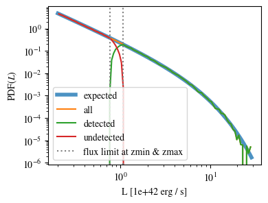
Check if the luminosity function is reproduced:
plt.figure(figsize=(4,3))
Ls = np.logspace(np.log10(lim.Lmin.to(luminosity_unit).value),
                 np.log10(np.nanmin([lim.Lmax.to(luminosity_unit).value, 1e6 * lim.Lmin.to(luminosity_unit).value])), 100)
n_bar_gal = quad(lim.luminosity_function, lim.Lmin.to(luminosity_unit).value, lim.Lmax.to(luminosity_unit).value)[0]
plt.plot(Ls, lim.luminosity_function(Ls) / n_bar_gal, label='expected', linewidth=4, alpha=0.8)
hist, bin_edges = np.histogram(lim.cat['luminosity'].to(luminosity_unit).value, bins=Ls, density=True)
hist_det, bin_edges = np.histogram(lim.cat['luminosity'][lim.cat['detected']].to(luminosity_unit).value, bins=Ls, density=True)
hist_undet, bin_edges = np.histogram(lim.cat['luminosity'][~lim.cat['detected']].to(luminosity_unit).value, bins=Ls, density=True)
plt.plot((Ls[:-1] + 0.5 * np.diff(Ls)), hist, label='all')
plt.plot(Ls[:-1] + 0.5 * np.diff(Ls), hist_det * (lim.N_gal_detected / lim.N_gal), label='detected')
plt.plot(Ls[:-1] + 0.5 * np.diff(Ls), hist_undet * (1-lim.N_gal_detected / lim.N_gal), label='undetected')

plt.axvline((lim.min_flux*(4*np.pi*lim.astropy_cosmo.luminosity_distance(lim.redshift+lim.delta_redshift)**2)).to(luminosity_unit).value,
              linestyle=':', color='gray')
plt.axvline((lim.min_flux*(4*np.pi*lim.astropy_cosmo.luminosity_distance(lim.redshift-lim.delta_redshift)**2)).to(luminosity_unit).value,
            linestyle=':', color='gray', label='flux limit at zmin & zmax')
plt.yscale("log")
plt.xscale("log")
plt.xlabel(f"L [{str(luminosity_unit)}]")
plt.ylabel(r"PDF($L$)")
plt.legend();
make sure that the selection function is working
print("input min_flux: {:e}\nmin flux of the detected galaxies: {:e}".format(lim.min_flux, np.min(lim.cat['flux'][lim.cat['detected']])))
print("Any galaxies that are below the detection limit? {}.".format(np.min(lim.cat['flux'][lim.cat['detected']]) < lim.min_flux))
input min_flux: 3.000000e-17 erg / (cm2 s)
min flux of the detected galaxies: 3.000023e-17 erg / (cm2 s)
Any galaxies that are below the detection limit? False.
Paint the intensity mesh
using the redshift-space positions.
If you want to work in real space, exchange RSD_Position with
Position.
intensity_mesh = lim.paint_intensity_mesh(position="RSD_Position");
Mesh assignment: finished 1/279646.
Mesh assignment: finished 100001/279646.
Mesh assignment: finished 200001/279646.
2023-07-14 14:15:13,108 simple WARNING: The smoothing length along or perpendicular to the LOS is smaller than the voxel size! You should consider using a larger smoothing length.
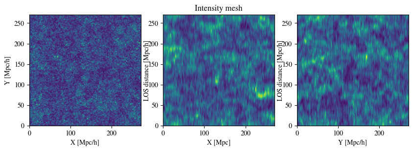
Plot the average intensity along the 3 different axes to visualize the smoothing:
fig = plt.figure(figsize=(10,3))

ax1 = fig.add_subplot(131)
ax1.imshow(np.mean(lim.intensity_mesh.value, axis=0),
           extent=[0,lim.box_size[1].value, 0, lim.box_size[2].value],
           origin='lower')
ax1.set_xlabel("X [Mpc/h]")
ax1.set_ylabel("Y [Mpc/h]")

ax2 = fig.add_subplot(132)
ax2.imshow(np.mean(lim.intensity_mesh.value, axis=1),
           extent=[0,lim.box_size[1].value, 0, lim.box_size[2].value],
           origin='lower')
ax2.set_xlabel("X [Mpc]")
ax2.set_ylabel("LOS distance [Mpc/h]", labelpad=-3)
ax2.set_title("Intensity mesh")

ax3 = fig.add_subplot(133)
ax3.imshow(np.mean(lim.intensity_mesh.value, axis=2),
           extent=[0,lim.box_size[1].value, 0, lim.box_size[2].value],
           origin='lower')
ax3.set_xlabel("Y [Mpc/h]")
ax3.set_ylabel("LOS distance [Mpc/h]", labelpad=-3);
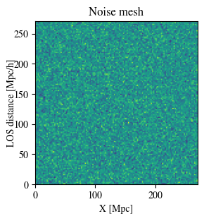
Get the intensity noise cube
lim.get_intensity_noise_cube()
plt.figure(figsize=(3,3))
plt.imshow(np.mean(lim.noise_mesh.value, axis=1),
           extent=[0,lim.box_size[1].value, 0, lim.box_size[2].value],
           origin='lower')
plt.xlabel("X [Mpc]")
plt.ylabel("LOS distance [Mpc/h]", labelpad=-3)
plt.title("Noise mesh");
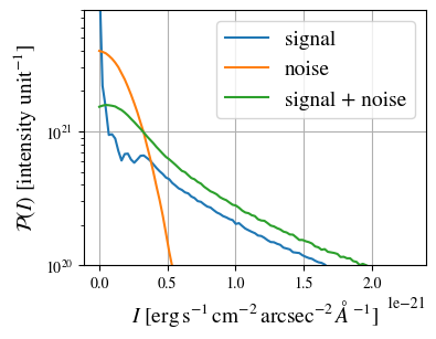
Plot the VID
Warning: numerical errors of the smoothing through FFT can cause some negative intensity values. This is especially true when the smoothing length is not much larger than the voxel size.
if lim.brightness_temperature:
    intensity_unit = u.uK / u.sr
    intensity_unit_str = r'$\mu$K'
else:
    try:
        lim.dnu
        intensity_unit = u.erg/u.s/u.cm**2/u.arcsec**2/u.Hz
        intensity_unit_str = r'$\mathrm{erg\, s^{-1}\, cm^{-2}\, arcsec}^{-2}\, \AA^{-1}$'
    except:
        intensity_unit = u.erg/u.s/u.cm**2/u.arcsec**2/u.angstrom
        intensity_unit_str = r'$\mathrm{erg\, s^{-1}\, cm^{-2}\, arcsec}^{-2}\, \AA^{-1}$'
log_I_bins = (np.linspace(0, 3, 100) * lim.mean_intensity).to(intensity_unit).value
vid, bin_edges = np.histogram(lim.intensity_mesh.to(intensity_unit).value, bins=log_I_bins, density=True)
vid_noise, bin_edges = np.histogram(lim.noise_mesh.to(intensity_unit).value, bins=log_I_bins, density=True)
vid_added, bin_edges = np.histogram((lim.intensity_mesh + lim.noise_mesh.to(lim.mean_intensity)).to(intensity_unit).value, bins=log_I_bins, density=True)
plt.figure(figsize=(4,3))
plt.plot(log_I_bins[:-1], vid, label='signal')
plt.plot(log_I_bins[:-1], vid_noise, label='noise')
plt.plot(log_I_bins[:-1], vid_added, label='signal + noise')

plt.yscale('log')
plt.xlabel(r'$I$ [{}]'.format(intensity_unit_str), fontsize=14)
plt.ylabel(r'$\mathcal{P}(I)$ [intensity unit$^{-1}$]', fontsize=14)
plt.grid()
plt.legend(fontsize=14)
plt.ylim(1e20, 8e21);
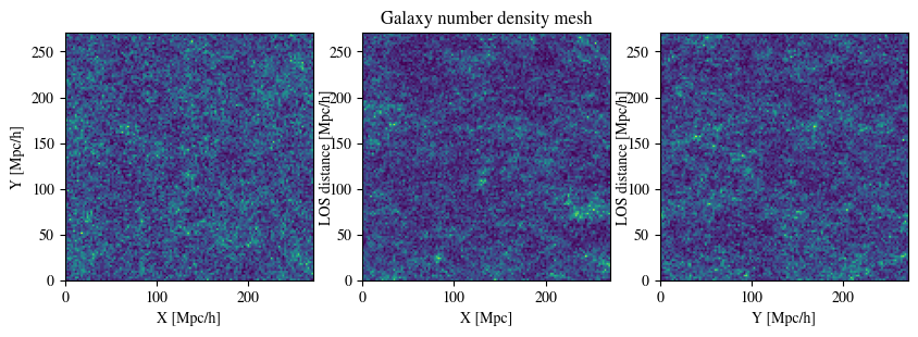
Generate the galaxy number density mesh:
lim.paint_galaxy_mesh(position="RSD_Position")

fig = plt.figure(figsize=(10,3))
ax1 = fig.add_subplot(131)
ax1.imshow(np.mean(lim.n_gal_mesh.value, axis=0),
           extent=[0,lim.box_size[1].value, 0, lim.box_size[2].value],
           origin='lower')
ax1.set_xlabel("X [Mpc/h]")
ax1.set_ylabel("Y [Mpc/h]")

ax2 = fig.add_subplot(132)
ax2.imshow(np.mean(lim.n_gal_mesh.value, axis=1),
           extent=[0,lim.box_size[1].value, 0, lim.box_size[2].value],
           origin='lower')
ax2.set_xlabel("X [Mpc]")
ax2.set_ylabel("LOS distance [Mpc/h]", labelpad=-3)
ax2.set_title("Galaxy number density mesh")

ax3 = fig.add_subplot(133)
ax3.imshow(np.mean(lim.n_gal_mesh.value, axis=2),
           extent=[0,lim.box_size[1].value, 0, lim.box_size[2].value],
           origin='lower')
ax3.set_xlabel("Y [Mpc/h]")
ax3.set_ylabel("LOS distance [Mpc/h]", labelpad=-3);
Mesh assignment: finished 1/55897.
Save the LognormalIntensityMock instance and catalog to files:
filename = os.path.join(
                lim.out_dir,
                "lognormal",
                "rsd",
                lim.outfile_prefix + "_lim_instance.h5",
            )
catalog_filename = os.path.join(
    lim.out_dir, "lognormal", lim.outfile_prefix + "_lognormal_rlz0.h5"
)
lim.save_to_file(filename=filename,
                              catalog_filename=catalog_filename)
Initiate a LognormalIntensityMock instance from a file:
lim = LognormalIntensityMock.from_file(filename = filename, catalog_filename = catalog_filename)
2023-07-14 14:15:17,289 simple WARNING: We extrapolate the values outside of the provided tabulated values of L.
Plot plt.loglog(Ls, lim.luminosity_function(Ls)) in a reasonable range to check the outcome!
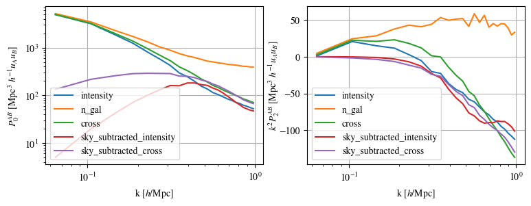
Calculate the power spectrum multipoles:
THe units \(u_A\) are \(u_\mathrm{g} = 1\) and \(u_I = \langle I \rangle\).
monopoles = {}
mean_ks = {}
quadrupoles = {}

for tracer in ["intensity", "n_gal", "cross", "sky_subtracted_intensity", "sky_subtracted_cross"]:
    mean_ks[tracer], monopoles[tracer], quadrupoles[tracer] = lim.Pk_multipoles(tracer=tracer, save=True)
/Users/maja/Documents/projects/intensity-mapping/simple/simple/tools_python.py:345: RuntimeWarning: invalid value encountered in true_divide
  return np.where(x != 0, j1(x) / x, 0.5)
fig = plt.figure(figsize=(9,3))
ax1 = fig.add_subplot(121)
for tracer in ["intensity", "n_gal", "cross", "sky_subtracted_intensity", "sky_subtracted_cross"]:
    ax1.plot(mean_ks[tracer], monopoles[tracer], label=tracer)

ax2 = fig.add_subplot(122)
for tracer in ["intensity", "n_gal", "cross", "sky_subtracted_intensity", "sky_subtracted_cross"]:
    ax2.plot(mean_ks[tracer], mean_ks[tracer]**2 * quadrupoles[tracer], label=tracer)

ax1.set_yscale("log")
ax1.set_xscale("log")
ax1.legend()
ax1.grid()
ax1.set_xlabel(r"k [$h$/Mpc]")
ax1.set_ylabel(r"$P_0^{AB}$ [Mpc$^3$ $h^{-1}u_A u_B$]")

ax2.set_xscale("log")
ax2.legend()
ax2.grid()
ax2.set_xlabel(r"k [$h$/Mpc]")
ax2.set_ylabel(r"$k^2 P_2^{AB}$ [Mpc$^3$ $h^{-1}u_A u_B$]", labelpad=-2);
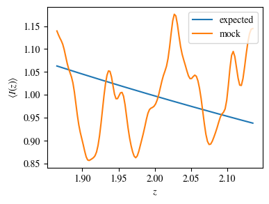
For the power spectrum, we need to calculate the mean intensity per
redshift and the mean galaxy number density per redshift. We can check
that it is working by calling
lim.mean_intensity_per_redshift(lim.redshift_mesh_axis, tracer='intensity')
or
lim.mean_intensity_per_redshift(lim.redshift_mesh_axis, tracer='n_gal')
plt.figure(figsize=(4,3))
plt.plot(lim.redshift_mesh_axis, lim.mean_intensity_per_redshift_mesh.to(lim.mean_intensity)[:,0,0], label='expected')
plt.plot(lim.redshift_mesh_axis, np.mean(lim.intensity_mesh, axis=(1,2)).to(lim.mean_intensity), label='mock')
plt.xlabel(r"$z$")
plt.ylabel(r"$\langle I(z)\rangle$")
plt.legend()
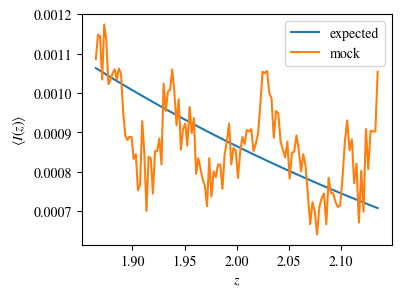
plt.figure(figsize=(4,3))
plt.plot(lim.redshift_mesh_axis, lim.mean_ngal_per_redshift_mesh.to(u.Mpc**-3)[:,0,0], label='expected')
plt.plot(lim.redshift_mesh_axis, np.mean(lim.n_gal_mesh, axis=(1,2)).to(u.Mpc**-3), label='mock')
plt.xlabel(r"$z$")
plt.ylabel(r"$\langle I(z)\rangle$")
plt.legend();
Run everything in one step
You can also do everything in one step if the input dictionary is complete:
lim.run()
[0.   0.   0.06] eV
{'ofile_prefix': 'mock', 'inp_pk_fname': '../tmp/mocks/inputs/mock_pk.txt', 'xi_fname': '../tmp/mocks/inputs/mock_Rh_xi.txt', 'pkg_fname': '../tmp/mocks/inputs/mock_pkG.dat', 'mpkg_fname': '../tmp/mocks/inputs/mock_mpkG.dat', 'cpkg_fname': '../tmp/mocks/inputs/mock_mpkG.dat', 'f_fname': '../tmp/mocks/inputs/mock_fnu.txt', 'z': 2.0, 'mnu': 0.06, 'oc0h2': 0.11934063901639999, 'ob0h2': 0.0224178568132, 'ns': 0.9645, 'lnAs': 3.094, 'h0': <Quantity 0.6766>, 'w': -1.0, 'run': 0.0, 'bias': 1.5, 'bias_mpkG': 1.0, 'bias_cpkG': 1.35, 'Nrealization': 1, 'Ngalaxies': 279657, 'Lx': 270.6403431715201, 'Ly': 270.6403431715201, 'Lz': 270.6403431715201, 'rmax': 10000.0, 'seed': 100, 'Pnmax': 128, 'losy': 0.0, 'losz': 0.0, 'kbin': 0.01, 'kmax': 0.0, 'lmax': 4, 'gen_inputs': True, 'run_lognormal': True, 'calc_pk': False, 'calc_cpk': False, 'use_cpkG': 0, 'output_matter': 0, 'output_gal': 1, 'calc_mode_pk': 0, 'out_dir': '../tmp/mocks/', 'halofname_prefix': '', 'imul_fname': '', 'num_para': 1, 'om0h2': 0.14175849582959998, 'om0': 0.30966, 'ob0': 0.04897, 'ode0': 0.6888463055445441, 'losx': 1.0, 'As': 2.2065162338947054e-09, 'aH': 100.27554429639554}
dir_name:  ../tmp/mocks/
../tmp/mocks/rsd
../tmp/mocks/realspace
dir_name:  ../tmp/mocks/inputs
../tmp/mocks/inputs/rsd
../tmp/mocks/inputs/realspace
dir_name:  ../tmp/mocks/lognormal
../tmp/mocks/lognormal/rsd
../tmp/mocks/lognormal/realspace
dir_name:  ../tmp/mocks/pk
../tmp/mocks/pk/rsd
../tmp/mocks/pk/realspace
dir_name:  ../tmp/mocks/coupling
../tmp/mocks/coupling/rsd
../tmp/mocks/coupling/realspace
time ~/Documents/projects/playground/lognormal_galaxies/eisensteinhubaonu/compute_pk ../tmp/mocks//inputs/mock 0.30966 0.6888463055445441 0.04897 0.6766 -1.0 0.9645 0.0 2.2065162338947054e-09 0.06 2.0
 Calculate the linear power spectrum using Eisenstein & Hu's transfer function
time ~/Documents/projects/playground/lognormal_galaxies/compute_xi/compute_xi ../tmp/mocks/inputs/mock ../tmp/mocks/inputs/mock_pk.txt 1037
 read in ../tmp/mocks/inputs/mock_pk.txt
time ~/Documents/projects/playground/lognormal_galaxies/compute_pkG/calc_pkG ../tmp/mocks/inputs/mock_pkG.dat ../tmp/mocks/inputs/mock_Rh_xi.txt 2 1.5 10000.0
time ~/Documents/projects/playground/lognormal_galaxies/compute_pkG/calc_pkG ../tmp/mocks/inputs/mock_mpkG.dat ../tmp/mocks/inputs/mock_Rh_xi.txt 2 1.0 10000.0
time ~/Documents/projects/playground/lognormal_galaxies/generate_Poisson/gen_Poisson_mock_LogNormal ../tmp/mocks/inputs/mock_pkG.dat ../tmp/mocks/inputs/mock_mpkG.dat 0 ../tmp/mocks/inputs/mock_mpkG.dat 270.6403431715201 270.6403431715201 270.6403431715201 128 279657 100.27554429639554 ../tmp/mocks/inputs/mock_fnu.txt 1.5 19094 60232 59629 ../tmp/mocks//lognormal/mock_lognormal_rlz0.bin ../tmp/mocks//lognormal/mock_density_lognormal_rlz0.bin 0 1
-------------beginning generate_poisson---------------------
Setting up the arrays.......
n0,n1,n2=128        128     128
size of Fourier grid is (n0,n1,n2)
(128,128,128)
Fourier resolution is 2.11438[Mpc/h]
Lx 270.64
Ly 270.64
Lz 270.64
kF0 0.023216
Generating mock density field in k-space
Note: The following floating-point exceptions are signalling: IEEE_UNDERFLOW_FLAG

real        0m0.014s
user        0m0.005s
sys 0m0.005s

real        0m0.035s
user        0m0.027s
sys 0m0.004s

real        0m0.022s
user        0m0.015s
sys 0m0.004s

real        0m0.023s
user        0m0.016s
sys 0m0.005s
Finished generating mock density field.
Doing FFT for density field.
Done FFT for density field.
Average of Log-normal density field  :-1.74366e-09
Variance of Log-normal density field :1568.33
Average of Log-normal density field  :-8.31441e-16
Variance of Log-normal density field :1.08298
Average of matter Log-normal density field :7.25929e-11
Variance of matter Log-normal density field :1197.7
Average of matter Log-normal density field :3.4615e-17
Variance of matter Log-normal density field :0.82705
density maximum = 153.52
density minimum = -0.997805
Average of density field: 0.00100348
Variance of density field: 2.26557
Doing FFT for the density field.
Calculating velocity field in Fourier space...
Doing FFT for the vx field.
Doing FFT for the vy field.
Doing FFT for the vz field.
Initializing random generater..
checkpoint 1
Ngalaxies 279657
checkpoint 2
checkpoint 3
checkpoint 4
final_array_length 3355884
checkpoint 5: allocated array.
Generating Poisson particles...........
ngalbar: 0.133351
checkpoint 6: starting nested for loops.
Total number of 279646 galaxies are generated!
min[vx] = -1681.87  max[vx] = 1623.85
avg[vx] = -0.427649 var[vx] = 51906.9
min[vy] = -1658.54  max[vy] = 1473.81
avg[vy] = 0.407441  var[vy] = 46194.3
min[vz] = -1979.67  max[vz] = 1422.05
avg[vz] = 0.207766  var[vz] = 57476.9
Final nPoisson: 279646
skip: calculate Pk
Saving to ../tmp/mocks/lognormal/mock_lognormal_rlz0.h5
Memory usage:  0.54898046875  GB.
Edges of the galaxy coordinates:
0.0001535301 270.64026
0.0003810556 270.63986
0.00022548102 270.63904
Overwriting Position in ../tmp/mocks/lognormal/mock_lognormal_rlz0.h5.
Overwriting Velocity in ../tmp/mocks/lognormal/mock_lognormal_rlz0.h5.
Saved to ../tmp/mocks/lognormal/mock_lognormal_rlz0.h5
real        0m0.198s
user        0m0.242s
sys 0m0.026s
Mesh assignment: finished 1/279646.
Mesh assignment: finished 100001/279646.
Mesh assignment: finished 200001/279646.
2023-07-14 14:15:21,679 simple WARNING: The smoothing length along or perpendicular to the LOS is smaller than the voxel size! You should consider using a larger smoothing length.
Mesh assignment: finished 1/55934.